Biologging devices often record information about an animal’s behavior using an inertial measurement unit (IMU) that collects acceleration, magnetometer, and/or orientation data. Because collecting these data can be battery- and storage-intensive, they are often recorded intermittently in rapid sets of samples at a fixed frequency, which we will refer to as bursts. These bursts of IMU measurements provide regular snapshots of an animal’s behavior and activity.
(Note that while some IMUs allow you to record data continuously for longer periods of time, we still use the term burst to refer to a distinct set of fixed-frequency IMU data samples, regardless of how long such a “burst” lasts.)
move2imu provides an R vector representation of these bursts so that
they can be easily manipulated, analyzed, and linked to other tracking
data—for instance, those stored in a move2 object. The
package currently supports three sensor types:
Each of these shares the same underlying structure. For the rest of this vignette, we will use acceleration data as an example.
Burst structure
You can create an acc vector from scratch by providing a
list of burst matrices (containing the raw acceleration data) and the
associated sampling frequency for those observations. Each burst can
contain up to three recording axes: X, Y,
and/or Z. Note that the frequency must be provided in
frequency units (in this case, "Hz"). move2imu uses the units package to
support unit manipulation.
raw_acc <- cbind(
  X = sin(1:30 / 10),
  Y = cos(1:30 / 10),
  Z = 1:30 / 10
)

a1 <- acc(
  bursts = list(raw_acc),
  frequency = units::as_units(40, "Hz")
)

a1
#> <acceleration[1]>
#> [1] (0.67 0.01 1.55)
#> # frequency: 40 [Hz]
The printed output of the vector shows the number of bursts as well as the mean value per axis for each burst. Internally, the raw data matrix is preserved.
Bursts can also be associated with a timestamp marking the start time of the burst:
a2 <- acc(
  bursts = list(
    cbind(X = sin(1:20 / 10), Y = cos(1:20 / 10)),
    cbind(X = sin(1:20 / 10 + 2), Y = cos(1:20 / 10 + 3))
  ),
  frequency = units::as_units(30, "Hz"),
  start = as.POSIXct(c("2026-06-01 00:00:00", "2026-06-01 00:01:00"), tz = "UTC")
)
Multiple acc vectors can be combined with
c(), even if their sampling frequency, axes, or other
properties vary:
a <- c(a1, a2)

a
#> <acceleration[3]>
#> [1] (0.67 0.01 1.55) (0.73 0.42)      (0.08 -0.52)
#> # frequency: 30 [Hz] - 40 [Hz]
Loading IMU data
Of course, in most cases you won’t be building bursts from scratch,
but will load these data from external sources. move2imu has been
designed to work in tandem with move2 and Movebank and will automatically
parse IMU data stored in one of Movebank’s standard storage formats (see
movebank_acc_colsets()).
Typically, data will be stored in a move2 object, which
contains the necessary timestamp and track ID metadata to correctly
parse IMU bursts. (You can also provide data as a
data.frame, but you will need to manually provide timestamp
and track ID metadata.)
For example, we’ll load a sample dataset of albatross tracks stored
as a move2:
# Load sample Movebank data into a `move2`
alb <- albatrosses()

alb
#> A <move2> with `track_id_column` "individual_local_identifier" and
#> `time_column` "timestamp"
#> Containing 9 tracks lasting on average 59.3 mins in a
#> Simple feature collection with 54 features and 21 fields (with 45 geometries empty)
#> Geometry type: POINT
#> Dimension:     XY
#> Bounding box:  xmin: -89.67882 ymin: -9.06721 xmax: -78.67636 ymax: -1.025846
#> Geodetic CRS:  WGS 84
#> # A tibble: 54 × 22
#>    sensor_type_id individual_local_identifier eobs_battery_voltage
#>  *        <int64> <fct>                                       [mV]
#>  1            653 4266-84831108                               3759
#>  2        2365683 4266-84831108                                 NA
#>  3        2365683 4266-84831108                                 NA
#>  4        2365683 4266-84831108                                 NA
#>  5        2365683 4266-84831108                                 NA
#>  6        2365683 4266-84831108                                 NA
#>  7            653 4261-2228                                   3720
#>  8        2365683 4261-2228                                     NA
#>  9        2365683 4261-2228                                     NA
#> 10        2365683 4261-2228                                     NA
#> # ℹ 44 more rows
#> # ℹ 19 more variables: eobs_fix_battery_voltage [mV],
#> #   eobs_horizontal_accuracy_estimate [m], eobs_key_bin_checksum <int64>,
#> #   eobs_speed_accuracy_estimate [m/s], eobs_start_timestamp <dttm>,
#> #   eobs_status <ord>, eobs_temperature [°C], eobs_type_of_fix <fct>,
#> #   eobs_used_time_to_get_fix [s], ground_speed [m/s], heading [°],
#> #   height_above_ellipsoid [m], timestamp <dttm>, visible <lgl>, …
#> Track features:
#> # A tibble: 9 × 52
#>   deployment_id  tag_id individual_id animal_life_stage attachment_type
#>         <int64> <int64>       <int64> <fct>             <fct>
#> 1       9472222 2911134       2911065 adult             tape
#> 2       9472220 2911111       2911067 adult             tape
#> 3       9472218 2911109       2911060 adult             tape
#> 4       9472214 2911130       2911066 adult             tape
#> 5       9472208 2911108       2911074 adult             tape
#> 6       2911178 2911132       2911094 adult             tape
#> 7       2911168 2911129       2911093 adult             tape
#> 8       2911167 2911127       2911092 adult             tape
#> 9       2911150 2911126       2911091 adult             tape
#> # ℹ 47 more variables: deployment_comments <chr>, deploy_on_timestamp <dttm>,
#> #   duty_cycle <chr>, deployment_local_identifier <fct>,
#> #   manipulation_type <fct>, study_site <chr>, tag_readout_method <fct>,
#> #   sensor_type_ids <chr>, capture_location <POINT [°]>,
#> #   deploy_on_location <POINT [°]>, deploy_off_location <POINT [°]>,
#> #   individual_comments <chr>, individual_local_identifier <fct>,
#> #   taxon_canonical_name <fct>, individual_number_of_deployments <int>, …
Then, to extract the acceleration data from this object, we simply
call as_acc():
a <- as_acc(alb)

a
#> <acceleration[54]>
#>  [1] <NA>              (1824.17 1913.83) (1904.3 1926.5)   (1823.27 1913.42)
#>  [5] (1826.7 1915.7)   (1719.07 1908.8)  <NA>              (1943.47 2028.05)
#>  [9] (1927.98 2013.72) (1926.7 2008.82)  (1940.97 2023.93) (1940.02 2021.87)
#> [13] (1969.07 2044.2)  <NA>              (1962.88 2033.35) (2062.08 2023.48)
#> [17] (2090.73 2025.83) (2083.92 2051.48) (1887.58 1927.13) <NA>
#> [21] (1846.38 1948.13) (1881.15 1938.03) (1841.58 2093.23) (1778.92 2129.55)
#> [25] (1812.17 1952.13) <NA>              (1790.4 1927.4)   (1811.85 1923.43)
#> [29] (1804.47 1935.05) (1811.45 1937.57) (2012.53 2227.17) <NA>
#> [33] (1970.52 2238.62) (2130.75 2082.43) (1997.18 2074.33) (2049.4 2060.38)
#> [37] (1975.93 1868.22) <NA>              (1920.02 2128.58) (1879.35 1920.62)
#> [41] (1927.5 1941.72)  (1949.27 1962.57) (1936.87 1918.93) <NA>
#> [45] (1672.52 1865.77) (1942.15 1922.33) (2072.85 1952.1)  (1617.97 1944.63)
#> [49] (1845.87 1921.13) <NA>              (1838.77 1929.6)  (1843.57 1929.52)
#> [53] (1852.25 1929.65) (1829.97 1932.28)
#> # frequency: 5 [Hz]
as_acc() automatically identifies the relevant
acceleration data in the albatross data and converts them into bursts
with associated frequencies and start timestamps.
By default, rows in the move2 with no acceleration data
receive missing (NA) acc bursts. This makes it
easy to keep acceleration bursts linked to other metadata stored in the
move2, like GPS location:
alb |>
  mutate(acceleration = a) |>
  select(acceleration)
#> A <move2> with `track_id_column` "individual_local_identifier" and
#> `time_column` "timestamp"
#> Containing 9 tracks lasting on average 59.3 mins in a
#> Simple feature collection with 54 features and 3 fields (with 45 geometries empty)
#> Geometry type: POINT
#> Dimension:     XY
#> Bounding box:  xmin: -89.67882 ymin: -9.06721 xmax: -78.67636 ymax: -1.025846
#> Geodetic CRS:  WGS 84
#> # A tibble: 54 × 4
#>         acceleration              geometry timestamp
#>                <acc>           <POINT [°]> <dttm>
#>  1                NA  (-78.67636 -9.06721) 2008-07-27 00:00:56
#>  2 (1824.17 1913.83)                 EMPTY 2008-07-27 00:00:56
#>  3   (1904.3 1926.5)                 EMPTY 2008-07-27 00:15:00
#>  4 (1823.27 1913.42)                 EMPTY 2008-07-27 00:30:00
#>  5   (1826.7 1915.7)                 EMPTY 2008-07-27 00:45:00
#>  6  (1719.07 1908.8)                 EMPTY 2008-07-27 01:00:00
#>  7                NA (-89.45139 -2.083909) 2008-07-27 00:00:15
#>  8 (1943.47 2028.05)                 EMPTY 2008-07-27 00:00:15
#>  9 (1927.98 2013.72)                 EMPTY 2008-07-27 00:15:00
#> 10  (1926.7 2008.82)                 EMPTY 2008-07-27 00:30:00
#> # ℹ 44 more rows
#> # ℹ 1 more variable: individual_local_identifier <fct>
#> Track features:
#> # A tibble: 9 × 52
#>   deployment_id  tag_id individual_id animal_life_stage attachment_type
#>         <int64> <int64>       <int64> <fct>             <fct>
#> 1       9472222 2911134       2911065 adult             tape
#> 2       9472220 2911111       2911067 adult             tape
#> 3       9472218 2911109       2911060 adult             tape
#> 4       9472214 2911130       2911066 adult             tape
#> 5       9472208 2911108       2911074 adult             tape
#> 6       2911178 2911132       2911094 adult             tape
#> 7       2911168 2911129       2911093 adult             tape
#> 8       2911167 2911127       2911092 adult             tape
#> 9       2911150 2911126       2911091 adult             tape
#> # ℹ 47 more variables: deployment_comments <chr>, deploy_on_timestamp <dttm>,
#> #   duty_cycle <chr>, deployment_local_identifier <fct>,
#> #   manipulation_type <fct>, study_site <chr>, tag_readout_method <fct>,
#> #   sensor_type_ids <chr>, capture_location <POINT [°]>,
#> #   deploy_on_location <POINT [°]>, deploy_off_location <POINT [°]>,
#> #   individual_comments <chr>, individual_local_identifier <fct>,
#> #   taxon_canonical_name <fct>, individual_number_of_deployments <int>, …
Input data formats
The Movebank data model supports several storage formats for acceleration data. However, move2imu handles this heterogeneity out of the box:
# Sample Movebank data
gul <- gulls()

as_acc(gul)
#> <acceleration[1239]>
#>    [1] <NA>                     (-97.75 323.55 1963.95)
#>    [3] <NA>                     <NA>
#>    [5] <NA>                     <NA>
#>    [7] <NA>                     <NA>
#>    [9] <NA>                     <NA>
#>   [11] <NA>                     <NA>
#>   [13] <NA>                     <NA>
#>   [15] <NA>                     <NA>
#>   [17] <NA>                     <NA>
#> ...
Even though the albatross and gulls data sources store their
acceleration data differently, because each adheres to the Movebank data
model, as_acc() seamlessly parses the data into a set of
acc burst matrices.
For more details about the ways Movebank stores acceleration data,
see movebank_acc_colsets().
Fine-tuning data import
move2imu also supports IMU data extraction from
data.frame objects. The workflow is identical to that for
move2 objects, except that you will need to specify a
vector of timestamps and track IDs separately (move2
objects store this metadata and provide it to as_*()
directly).
x <- data.frame(
  acceleration_x = c(1, 2, 3, 4),
  acceleration_y = c(5, 6, 7, 8),
  acceleration_z = c(9, 10, 11, 12),
  timestamp = as.POSIXct("2024-01-01", tz = "UTC") + seq(0, 0.3, by = 0.1),
  id = "tag_1"
)

as_acc(x, timestamp = x$timestamp, track_id = x$id)
#> <acceleration[4]>
#> [1] (2.5 6.5 10.5) <NA>           <NA>           <NA>
#> # frequency: 10 [Hz]
Further, if your data are stored using column names that don’t adhere
to the Movebank data model, you can still use as_acc() to
load them, provided that the data themselves are stored in a
recognizable format (see imu_colset()). Use
imu_colset() to define the column names that correspond to
each axis of acceleration data in your input data source:
# The same samples, under custom column names
names(x)[1:3] <- c("acc_x", "acc_y", "acc_z")

as_acc(
  x,
  colset = imu_colset(x = "acc_x", y = "acc_y", z = "acc_z"),
  timestamp = x$timestamp,
  track_id = x$id
)
#> <acceleration[4]>
#> [1] (2.5 6.5 10.5) <NA>           <NA>           <NA>
#> # frequency: 10 [Hz]
Exploring bursts
For a quick summary of an IMU vector, use summary().
This shows the range of several key burst properties as well as the
quantiles of the inter-burst time intervals and the actual recorded
burst values.
a <- as_acc(albatrosses())

summary(a)
#> 54 acc bursts (9 NA)
#> from 2008-07-27 00:00:14 to 2008-07-27 01:00:00 UTC
#>
#> Axes: XY (45)
#> Frequencies: 5 -- 5 [Hz]
#> Samples per burst: 60 -- 60
#> Durations: 12 -- 12 [s]
#> Intervals: [ -3598 / 833 / 888 / 888 / 891 ] [s]  (min/Q1/med/Q3/max)
#>
#> Values:  [ 1462 / 1875 / 1936 / 2010 / 2988 ]  (min/Q1/med/Q3/max)
#> Units:   NULL
For a more detailed look at these properties, you can use move2imu’s dedicated accessors. For instance:
# Number of samples per burst
n_samples(a)
#>  [1] NA 60 60 60 60 60 NA 60 60 60 60 60 60 NA 60 60 60 60 60 NA 60 60 60 60 60
#> [26] NA 60 60 60 60 60 NA 60 60 60 60 60 NA 60 60 60 60 60 NA 60 60 60 60 60 NA
#> [51] 60 60 60 60

# Burst duration, in seconds
burst_dur(a)
#> Units: [s]
#>  [1] NA 12 12 12 12 12 NA 12 12 12 12 12 12 NA 12 12 12 12 12 NA 12 12 12 12 12
#> [26] NA 12 12 12 12 12 NA 12 12 12 12 12 NA 12 12 12 12 12 NA 12 12 12 12 12 NA
#> [51] 12 12 12 12

# Check whether all bursts have same frequency, samples, axes, units
is_uniform(a)
#> [1] TRUE

# and more...
If you need to operate on the burst data or metadata directly, they can easily be accessed as well:
bursts(a)
#> <acc_list[54]>
#> [[1]]
#> NULL
#>
#> [[2]]
#>          X    Y
#>  [1,] 1856 1900
#>  [2,] 1816 1931
#>  [3,] 1812 1902
#>  [4,] 1826 1920
#> ...

freqs(a)
#> Units: [Hz]
#>  [1] NA  5  5  5  5  5 NA  5  5  5  5  5  5 NA  5  5  5  5  5 NA  5  5  5  5  5
#> [26] NA  5  5  5  5  5 NA  5  5  5  5  5 NA  5  5  5  5  5 NA  5  5  5  5  5 NA
#> [51]  5  5  5  5

starts(a)
#>  [1] NA                        "2008-07-27 00:00:56 UTC"
#>  [3] "2008-07-27 00:15:00 UTC" "2008-07-27 00:30:00 UTC"
#>  [5] "2008-07-27 00:45:00 UTC" "2008-07-27 01:00:00 UTC"
#>  [7] NA                        "2008-07-27 00:00:15 UTC"
#>  [9] "2008-07-27 00:15:00 UTC" "2008-07-27 00:30:00 UTC"
#> [11] "2008-07-27 00:45:00 UTC" "2008-07-27 01:00:00 UTC"
#> [13] "2008-07-27 00:00:55 UTC" NA
#> [15] "2008-07-27 00:15:00 UTC" "2008-07-27 00:30:00 UTC"
#> [17] "2008-07-27 00:45:00 UTC" "2008-07-27 01:00:00 UTC"
#> [19] "2008-07-27 00:00:50 UTC" NA
#> ...
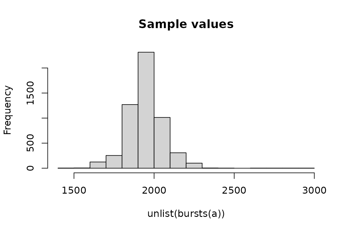
These can be used to easily explore the distributions of these properties:
# Distribution of inter-burst intervals
hist(burst_intervals(a), main = "Burst intervals (s)")
Plotting sampling effort
Many tags change their sampling settings over the course of a study.
To visualize how the IMU data were sampled, use
plot_sampling_effort(). This can reveal periods where
different sensors or tracks collected data simultaneously, where tags
stopped and started collecting data, and how densely certain time ranges
were sampled.
track_ids <- mt_track_id(albatrosses())

plot_sampling_effort(acc = a, ids = track_ids)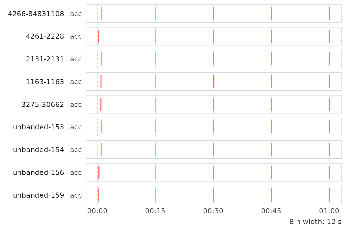
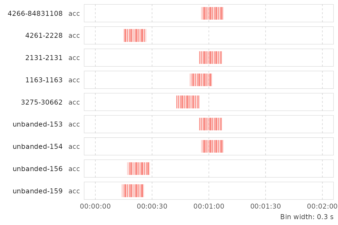
Modify the width of the aggregation bins and the plot’s time range to explore time periods in more detail:
start <- as.POSIXct("2008-07-27 00:00:00", tz = "UTC")
end <- as.POSIXct("2008-07-27 00:02:00", tz = "UTC")
width <- units::set_units(0.3, "s")

plot_sampling_effort(
  acc = a,
  ids = track_ids,
  bin_width = width,
  from = start,
  to = end
)
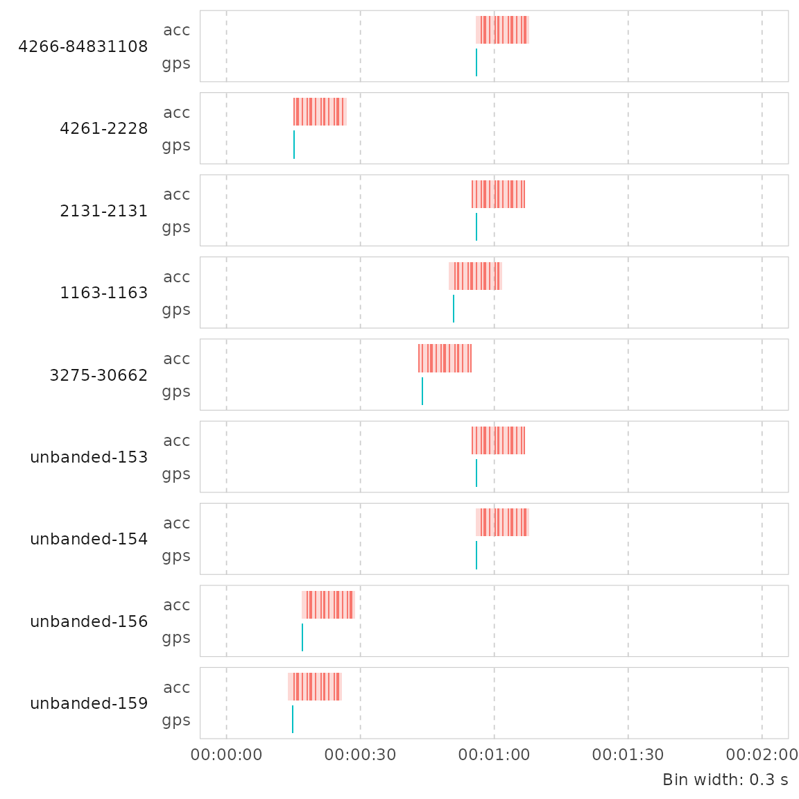
plot_sampling_effort() accepts both imu
objects as well as timestamp vectors, so you can also plot other sensors
based on their recorded timestamps (e.g. GPS coordinates):
# Mask out timestamps to get only those where a GPS location was recorded
gps <- replace(mt_time(albatrosses()), sf::st_is_empty(albatrosses()), NA)

plot_sampling_effort(
  acc = a,
  gps = gps,
  ids = track_ids,
  bin_width = width,
  from = start,
  to = end
)
Plotting IMU traces
You can also plot the values recorded by an IMU vector over time with
plot_imu_trace(). This produces an interactive dygraph that
you can zoom into with the mouse:
a <- as_acc(gulls())

plot_imu_trace(a)
You can also pass a single burst (or a subset) for a focused view — here, the wing beats are clearly visible on the Z axis:
plot_imu_trace(a[422])The plot is returned unstyled. Additional arguments are passed to
dygraphs::dygraph() and additional dygraphs
layers can be added to the output plot. For instance, to add axis labels
and ensure times are labeled in UTC instead of the browser’s local time
zone:
plot_imu_trace(a[422], main = "Wing beats", ylab = "Acceleration (g)") |>
  dygraphs::dyOptions(labelsUTC = TRUE)
Next steps
If your data are stored as raw ADC values rather than physical units, see the calibration vignette to learn how to convert them.
See the programming with bursts
vignette for a demonstration of how to compute values from
acc bursts and link them back to GPS coordinates in a
move2 object.